Hash
Hash
Hash란 임의의 크기를 가진 데이터를 고정된 크기의 데이터로 변환시키는 것을 말한다.
1차원 배열 형태의 Hash Table을 사용한다.
평균적으로 삽입, 삭제, 검색 시에 O(1) 의 시간이 걸린다.
Hash를 왜 사용할까?
1차원 배열을 사용하여 index를 통해 O(1)의 시간으로 저장공간에 접근하고자 한다.
[1, 100, 10, 9879] 라는 key값들을 1차원 배열을 사용하여 저장하기 위해서 아래 세 가지 방법을 비교해보자.
// 1번 : 단 4개의 저장공간만 사용하지만, 9879 라는 값을 찾으려면 O(n)의 시간이 필요하다.
int n = 4;
int[] arr = new int[n];

arr[0] = 1;
arr[1] = 100;
arr[2] = 10;
arr[3] = 9879;
// 2번 : 9879 라는 값을 찾으려면 O(1)의 시간만에 찾을 수 있지만, 9879개의 저장공간이 필요하다.
int n = 9879;
int[] arr = new int[n+1];

arr[1] = 1;
arr[100] = 100;
arr[10] = 10;
arr[9879] = 9879;
// 3번 : Hash Function 'h(x) = x mod 4' 을 사용한다.
//       9879 라는 값을 찾기위해 h(x)만 알고 있다면 O(1)의 시간만에 찾을 수 있다.
//       모든 데이터를 저장하는데 단 4개의 저장공간만 사용했다.
int n = 4;
int[] hashTable = new int[n];

hashTable[h(1,n)] = 1;         // h(1,n) = 1
hashTable[h(100,n)] = 100;     // h(100,n) = 0
hashTable[h(10,n)] = 10;       // h(10,n) = 2
hashTable[h(9879,n)] = 9879; // h(9879,n) = 3

...

int h(int x, int n) { return x % n; } // Hash Function
3번에서 Hash Function을 사용하여 임의의 값을 고정된 크기의 데이터로 변환했다.
변환된 값을 Hash Table(1차원 배열)의 index로 사용하였다.
그래서 효율적인 메모리 사용와 빠른 탐색이 가능하다.
그 외에도 보안의 목적으로 Hash를 많이 활용하지만 이 글에서는 다루지 않으며,
Java에서의 Hash를 활용한 HashSet, HashMap 등의 자료구조로 이어진다.
Hash Function : h(x)
hash function maps a big numbers or string to a small integer that can be used as index in hash table.
Hash Function은 큰 숫자 또는 문자열을 Hash Table에서 인덱스로 사용할 수있는 작은 정수로 매핑한다.
ex ) Division Method
h(x) = x mod m
m = table size =  7, x1 = 9864567654
h(x1) = 9864567654 mod 7 = 4
Collision (충돌)
Two keys resulting in same value. if (h(x1) == h(x2)) Collision!
두 개 이상의 key 값의 Hash Function의 결과가 중복되면 Collision이 발생한다.
good h(x) should be Efficiently Computable and Uniformly distribute the keys.
※ Efficiently Computable = Easy and Quick = Simple
좋은 Hash Function은 효율적인 계산이 가능하고 key가 균등하게 나타나도록 해야한다. (Simple Uniform Hash)
그러므로 Collision(충돌)을 덜 일으켜야 한다.
Hash Table
Direct Addressing Table
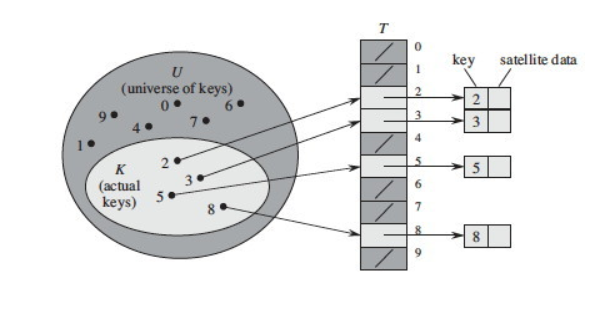
universe of keys(전체 key의 개수)와 Hash Table의 크기가 동일하기 때문에 Collision(충돌)이 발생하지 않는다.
하지만, actual keys(실제 사용하는 key의 개수)가 universe of keys 보다 적기 때문에 메모리 효율성이 떨어진다.
Load Factor
보통의 경우 Direct Addressing Table 보다는 Hash table의 크기(m)이 실제 사용하는 keys의 개수(n) 보다 적은 Hash Table을 사용한다.
이 때, n/m 을 load factor라고 한다.
Direct Addressing Table의 load factor는 1 이하이다.
load factor가 1보다 클 경우 Collision(충돌)이 발생한다.
Collision Handling
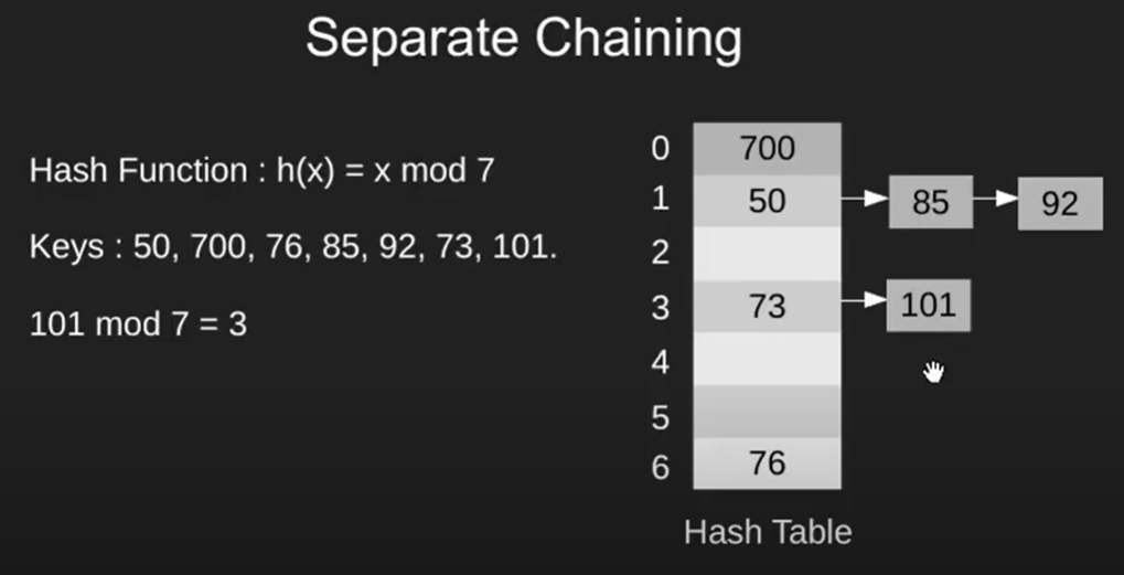
1. Separate Chaning
The idea is to make each cell of hash table point to a linked list of records that have same hash function value.
Hash Table의 각 cell (bucket) 을 linked list로 만든다.
Linked list는 동일한 h(x) 결과 값을 가진 records 들을 순차적으로 저장한다.
Advantages :
- Simple to implement.
확장성이 용이하다. 데이터의 삽입과 삭제가 편하다. - Hash table never fills up, we can always add more elements to chain.
- Less sensitive to the hash function or load factors.
Hash function 이나 n에 영향을 덜 받는다. (그러므로 load factors에 영향을 덜 받는다고 할 수 있다.)
Hash table이 가득 차는 경우가 거의 없고 n의 증가에 따라 성능저하가 Linear 하게 나타난다. - It is mostly used when it is unknown how many and how fequently keys may be inserted or deleted.
삽입, 삭제 빈도를 알수없는 경우에 주로 사용된다.
Disadvantages :
- Cache performance of chaining is not good as keys are stored using linked list.
- If the chain becomes long, then search time can become O(n) in worst case.
Linked list를 이용하므로 linked list의 단점을 그대로 받는다.
체인이 길어지면 최악의 경우 검색시간이 O(n)까지 걸릴 수 있다.
Cache performance가 좋지 않다.
참고 - Cache performance - Uses extra space for links.
Hash table space 외에도 linked list를 위한 별도의 space 가 필요하다. - Wastage of Space.
Hash table에 공간이 많이 남았는데 linked list에만 records를 채우다보면 공간이 낭비될 수 있다.
Time Complexity :
n = number of keys stored in table
m = number of slots in table (table size)
a = Average keys per slot or load factor = n/m

Expected time to insert/search/delete
O(1 +a)
2. Open Addressing
All elements are stored in the hash table itself.
모든 데이터를 Hash Table 자체에 저장한다.
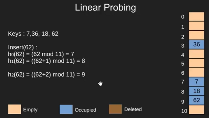
1) Liner Probing
충돌이 발생할 경우 i 칸 씩 이동.
hi(x) = (h(x)+i) mod m. (m = table size)

if h0 = (h(x) + 0) mod m is full, we try for h1
if h1 = (h(x) + 1) mod m is hull, we try for h2
and so on...
insert
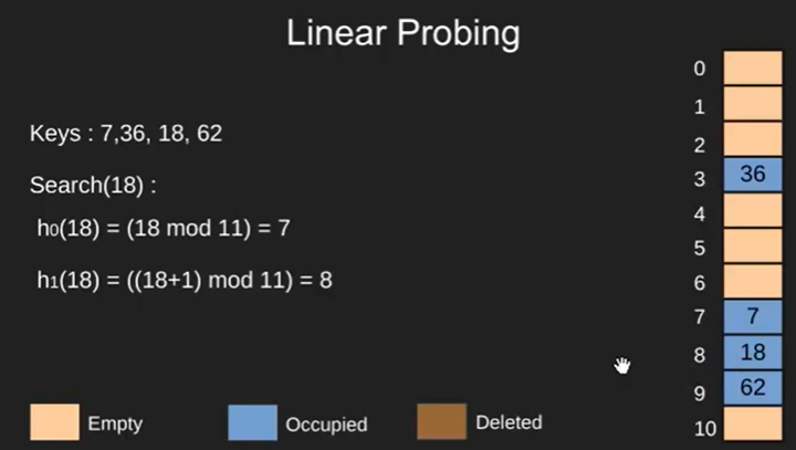
Search
Delete
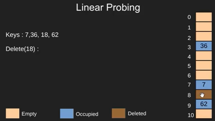
if we simply delete a key, so here we make a note that, we can insert a key at a slot with deleted state but search operation should not stop on this slot.
record가 삭제된 slot에 DEL 표시를 하는 등의 방법으로 해당 slot에서 검색이 중단되지 않도록 해야한다.
예를 들어, h(7) = h(18) = h(62) = 7 이다. 18을 삭제한 뒤 62를 검색하려고 했을 때, 삭제된 slot에 아무런 표시없이 비어있다면 62를 찾지 못하고 검색이 중단될 것이다.
2) Quadratic probing
충돌이 발생할 경우 i^2 칸 씩 이동.
hi(x) = (h(x) + i^2) mod m. (m = table size)

if h0 = (h(x) + 0) mod m is full, we try for h1
if h1 = (h(x) + 1) mod m is hull, we try for h2
if h2 = (h(x) + 4) mod m is hull, we try for h3
and so on...
Challenges in Linear Probing and Quadratic probing :
- Primary Clustering: One of the problems with linear probing is Primary clustering, many consecutive elements form groups and it starts taking time to find a free slot or to search for an element.
- Secondary Clustering: Secondary clustering is less severe, two records only have the same collision chain (Probe Sequence) if their initial position is the same.
참고 - Primary Clustering and Secondary Clustering
3) Double hasing
해시 함수를 2개 사용하며, 충돌이 발생할 경우 i * h(x) 칸 씩 이동.
hi(x) = (h(x) + i * h'(x)) mod m. (m = table size)

if h0 = (h(x) + 0) mod m is full, we try for h1
if h1 = (h(x) + 1 * h'(x)) mod m is hull, we try for h2
if h2 = (h(x) + 2 * h'(x)) mod m is hull, we try for h3
and so on...
Time Complexity :
n = number of keys stored in table
m = number of slots in table (table size)
a = load factor = n/m (< 1)

Expected time to inser/search/delete
O(1/(1-a))
Comparison V.1
| Linear Probing | Quadratic Probing | Double Hashing |
|---|---|---|
| Best Cache Performance | Average Cache Performance | Poor Cache Performance |
| Suffers from clustering | Suffers a lesser clustering than linear probing | No Clustering |
| Easy to implement | Requires more computation time |
Comparison V.2
| Linear Probing | Quadratic Probing | Double Hashing | |
|---|---|---|---|
| Cache Performance | 좋음 | 평균적 | 나쁨 |
| Clustering Issue | 나쁨 | Linear Probing보단 덜함 | 없음 |
| Computaion Time | 좋음 | 나쁨 |
NEXT…
Hashing in Java
- HashCode
- HashMap
- HashSet
Reference
GeeksforGeeks - Hashing, Set 1 (Introduction) + YouTube
GeeksforGeeks - Hashing, Set 2 (Separate Chaining) + YouTube